OpenCell basic model building tutorial

About this tutorial

This tutorial is based on the Getting started with CellML tutorial by Mike Cooling, in which COR is used to build a simple CellML model. In this tutorial, OpenCell will be used to build a very similar model. This tutorial also contains material written by Catherine Lloyd and James Lawson.

By following this tutorial you will learn how to create a simple, functional CellML model from scratch using a CellML editing and simulation environment called OpenCell, and how to display the results of simulating this model on a graph.

Creating a new model

We'll begin by defining some equations and parameters that we would like to use CellML to describe. Let's say we want to model the simple chemical reaction shown below:

Using mass action kinetics, we might model this as:

Where:

[A], [B] and [C] are the concentrations of the reaction species, k_f and k_b are rate constants and J is a flux.

To create this model in CellML, we will use two components: an environment component to contain the time variable, and a flux component to contain the reaction. We will use seven variables: time, the reaction species A, B, and C, the rate constants k_f and k_b, and the flux J. There will be a connection between the two components to pass the time variable.

Although the best description of elements within a CellML model can be found within the CellML 1.1 Specification, a brief comment on components and connections is in order here.

Every variable in a CellML model is defined within a component. These components allow a modeller to organize and group variables and equations into modules. There is no ordained way to do this, so a modeller may in fact choose to create only one component and put everything in the model within it, but usually the components represent discrete processes or entities within the model, such as protein interactions in a signal transduction model. This is useful both because it keeps the model neat and aids conceptualization and because it facilitates the creation of reusable modules.

Connections allow the modeller to map variables within different components to each other. This means that a variable may be defined by an equation in one component and mapped to another component to be used. Because the derivative of each ODE in this model needs to be taken with respect to time, the variable that tracks time needs to be defined once and mapped to each component.

When you first load OpenCell, it will look something like this (depending on your operating system and monitor resolution):

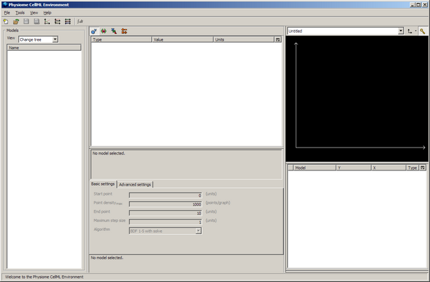
The window is divided into four sections; the model selector pane, tree view pane, interaction pane, and the graph pane. For more information about the OpenCell interface, refer to the manual - also available from the Help menu from within OpenCell.

Create a model

Click on the first button on the toolbar (new model) or go to the File menu and select New. A window titled Create new model will appear, asking for a name and a CellML version for your new model. Type in tutorial_model, and select CellML 1.1 for the CellML version. Press enter, or click on OK. You will now have a model called tutorial_model visible in the model selector pane.

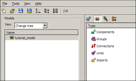
Now switch to the show complete model structure view in the tree view pane, using the second button on the tree view pane toolbar. This view is the main view you will use to edit models in OpenCell.

You will see a list of items in the tree view pane; Components, Groups, Connections, Units, and Imports.

Click on the Save button (the diskette icon) or select Save from the File menu. Give your file the name tutorial_model.cellml and save it in your chosen folder. Save regularly during this tutorial.

Making new components

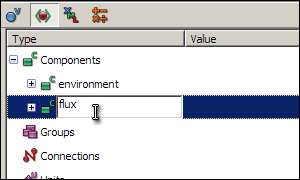
You are going to create two components; one called environment to contain the global variable time, and another called flux to contain the variables and equations for the reaction.

To create a new component, right click on the green icon labelled Components, and select New from the context menu. A component called New_component will appear below Components - select the name of this component, type in environment (in place of New_component) and press enter. Now create another component, and rename it to flux.

Creating variables

You will now create the variables for the model, within the appropriate components. First create the time variable: right click on the environment component's icon in the tree view (the green rectangle with a C, labelled environment) and select New variable from the context menu. Re-name the variable from New_variable to time.

The other six variables should be created in the flux component. Create the variables A, B, C, kf, kb and J under the flux component. Some of these variables will require initial values. These can be entered in the Value field of the tree view. Enter values of 2, 3, and 0 for the variables A, B, and C respectively. These values are the initial concentrations of these three species. The rate constant variables kf and kb should be given values of 0.15 and 0.5.

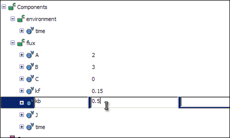
You will also need to create the variable time in the flux component, which will later be connected to the time variable in the environment component. Variables that are connected must appear in both of the connected components.

Defining units

All variables and numbers in a CellML model must be associated with units. OpenCell has a library of pre-defined units, which includes all base and derived SI units. First, associate the unit second with the time variable - click on the Units field of the time variable in the tree view, and select second from the list of pre-defined units.

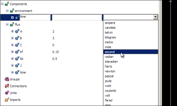
The other units used in this model will have to be defined, as they do not appear in the list of pre-defined units. The concentration of the three reaction species are in units of micromoles per litre, or micromolar; the flux will be in units of micromolar per second. The two reaction rates will have units of per micromolar per second (for kf) and per second (for kb).

These units are made up of combinations of SI units, modified by prefixes, multipliers, offsets, and exponents. For example, the unit micromolar is made up of mole with a prefix of -6 (micro) combined with litre with an exponent of -1; micromoles per litre.

To define the unit micromolar, right click on the Units icon in the tree view and select New unit from the context menu. Rename this unit uM, and make sure that the type of unit is Derived. Now right click on the icon for uM and select New unit again from the context menu. Select mole from the list of units next to the yellow triangular unit node icon. To make these micromoles, enter a value of -6 into the Prefix text field, or select micro from the list of prefixes. Right click again on the uM icon, and select New unit again. For this new unit, select litre from the list of pre-defined units. To make this per litre, enter a value of -1 into the exponent field of the litre unit.

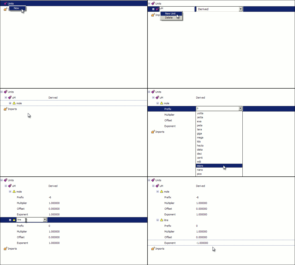
To define the remaining units follow the procedure above, using the components of each unit.

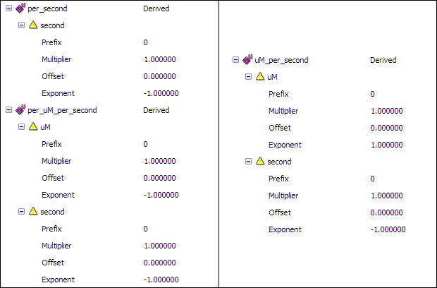
• The per_second unit is defined as a second unit with an exponent of -1 .
• uM_per_second is defined using uM combined with the second unit with an exponent of -1.
• per_uM_per_second is defined using uM with an exponent of -1, combined with the second unit with an exponent of -1.

This will give you the following unit definitions:

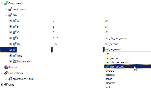
Now that you have defined all the required units, you can associate them with the variables. Click on the units field of each variable, and select the appropriate unit for each of the variables.

A: uM

B: uM

C: uM

kf: per_uM_per_second

kb: per_second

J: uM_per_second

Creating equations

Now you will enter the model equations. These are created within the appropriate component, in this case the flux component. Right click on the icon for the component in the tree view, and select New maths from the context menu. An icon labelled Mathematics will appear; right click on it and select New equation from the context menu. Do this four times to create four equations.

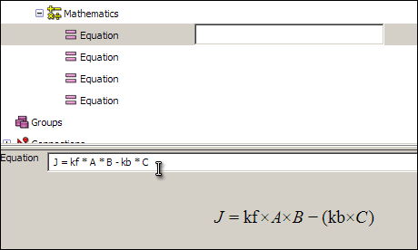
Click on the first equation, and in the text box (which will initially read <no operator yet>) enter the following equation:

J = kf * A * B - kb * C

For the second, third, and fourth equations, enter:

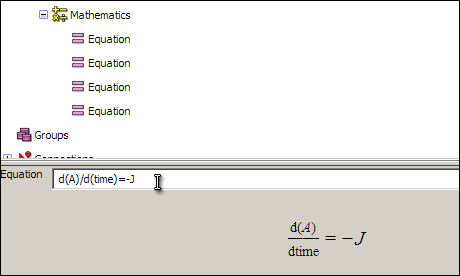
d(A)/d(time)=-J

d(B)/d(time)=-J

d(C)/d(time)=J

After you have entered the equation, selecting it will cause a formatted version of the equation to appear in the interaction pane below the tree view. This will only if you have entered an equation in a way that OpenCell is able to interpret. The input format is an editable form of MathML and is similar to the format for a basic command-line calculator tool.

Creating connections

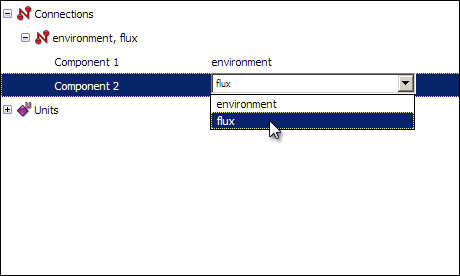
Finally, you will need to create a connection between the two components, to pass the time variable from the environment component to the flux component. As we mentioned previously, connections allow variables which have been defined in one component to be used within another component. To create a connection, right click on the red Connections icon in the tree view, and select New from the context menu. Expanding the newly created connection will show you two items named Component 1 and Component 2. Select environment and flux respectively from the drop-down menus.

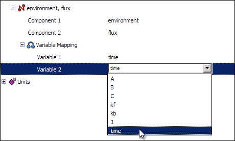
Now, right click on the connection labelled environment, flux and select New variable mapping from the context menu. Expanding the new variable mapping will show you two items labelled Variable 1 and Variable 2. You want to map the variable time from the environment component onto time from the flux component, so select time in both of the fields.

For this connection to function, you must also set the Public Interface of the time variables correctly in for each component. Do this by first expanding the time variable in the environment component, and then selecting Out from the Public Interface drop-down menu.

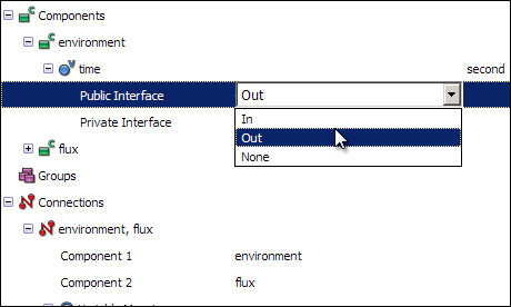
In the same way, change the Public interface of the time variable in the flux component to In.

Validating the model

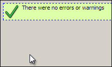
Validating the model will help you to identify and locate any errors you might have made in building your model.

To validate the model, right click on the model name in the model selector panel on the left, and select Validate from the context menu. If there are no errors, a message will appear in the far right hand pane of the OpenCell window, the graph pane.

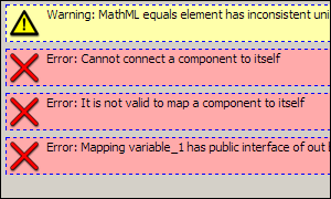
If there were errors, messages will appear describing the errors found. Double-clicking on the error messages will take you to the part of the model where the error was detected. Take note that you must be in the complete model structure view for this error highlighting function to work correctly. Here is an example of what these error messages might look like: Here is an example of what these error messages might look like:

Running a simulation

Our model is now validated and ready to simulate. Save the model now, and then click on the Display integration pane button (the last button on the toolbar, with the letters dt,) to make the integration pane visible. You have to close and re-load the model before the integration pane becomes available. The integration pane should look something like this:

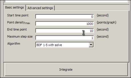
Click on the large Integrate button, and wait until the message Integration complete appears in the integration pane. The Integrate button will change to the Export CSV button. This button allows you to save the results of the simulation as comma separated values, for loading into other applications. You now have results for the model which you can display in the graph pane.

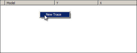
Right click in the graph trace control area in the grap pane, and select New Trace from the context menu.

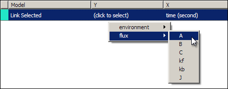
A new trace entry will appear in the listing. Click on the X column where it says (click to select) and select environment, time from the cascading menu. Do the same for the Y column and select flux, A.

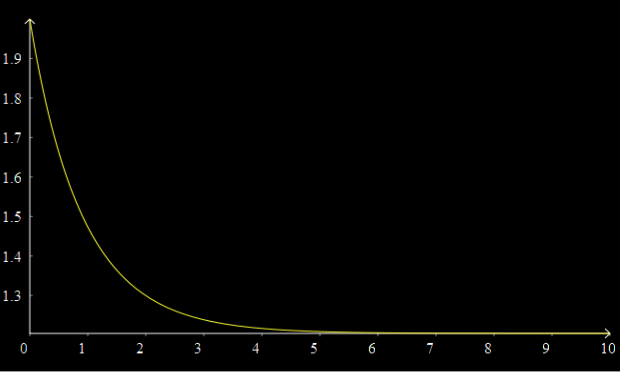
A graph should now appear above, showing the concentration of A decaying over time to its equilibrium value.

Add more traces to the graph; right click in the graph controls and select New Trace to create three more traces. The new traces will automatically have time selected as the X axis variable, although you can of course change this if you wish by clicking on it and selecting a different variable. Select B, C, and J as the other three Y variables for the other traces. You should now have a graph that looks something like this:

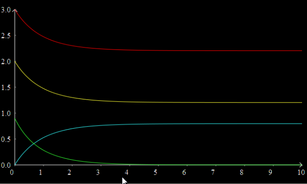
You can change the colour of individual traces by clicking on the coloured block in the graph controls and selecting a colour from the pop up palette.

This concludes the tutorial. Please refer to the manual and other tutorials for more information.